Suggests the mice options to perform multiple imputation, based on the set of imputation models (one for each partially observed variable) specified by calls to checkModSpec and the proportion of complete records. Optionally, if a dataset is supplied, diagnostic plots are created based on the proposed 'mice' options.
Usage
proposeMI(
  mimodobj,
  prop_complete = NA,
  data = NULL,
  plot = TRUE,
  plotprompt = TRUE,
  message = TRUE
)
Arguments
- mimodobj
An object, or list of objects, of type 'mimod', which stands for 'multiple imputation model', created by a call to checkModSpec
- prop_complete
Optionally, the proportion of complete records, specified as a number between 0 and 1. This is only required if a dataset is not specified. If a dataset is specified, the proportion of complete records will be calculated based on all columns included in the dataset.
- data
Optionally, a data frame containing all the variables required for imputation and the substantive analysis; if stratification variable(s) are included in the 'mimod' object(s), these will be carried over to 'midoc' functions 'doMImice' and 'doMNARmice' and multiple imputation will be performed for each subset of the data determined by the values of the stratification variable(s)
- plot
If TRUE (the default), and a dataset is supplied, displays diagnostic plots for the proposed 'mice' call; use plot=FALSE to disable the plots
- plotprompt
If TRUE (the default), and a dataset is supplied, the user is prompted before the second plot is displayed; use plotprompt=FALSE to remove the prompt and display all plots at the same time
- message
If TRUE (the default), displays a message describing the proposed 'mice' options; use message=FALSE to suppress the message
Value
An object of type 'miprop', which can be used to run 'mice' using the proposed options, plus optionally, a message and, if a dataset is supplied, diagnostic plots describing the proposed 'mice' options
Examples
# First specify each imputation model as a 'mimod' object
## (suppressing the message)
mimod_bmi7 <- checkModSpec(formula="bmi7~matage+I(matage^2)+mated+pregsize",
family="gaussian(identity)",
data=bmi,
message=FALSE)
 mimod_pregsize <- checkModSpec(
formula="pregsize~bmi7+matage+I(matage^2)+mated",
family="binomial(logit)",
data=bmi,
message=FALSE)
#> Registered S3 method overwritten by 'car':
#> method from
#> na.action.merMod lme4
mimod_pregsize <- checkModSpec(
formula="pregsize~bmi7+matage+I(matage^2)+mated",
family="binomial(logit)",
data=bmi,
message=FALSE)
#> Registered S3 method overwritten by 'car':
#> method from
#> na.action.merMod lme4
 # Display the proposed 'mice' options
## When specifying a single imputation model
proposeMI(mimodobj=mimod_bmi7,
data=bmi)
#> Based on your proposed imputation model and dataset, your mice() call
#> should be as follows:
#>
#> mice(data = bmi , # You may need to specify a subset of the columns in
#> your dataset; if you specified stratification variable(s) in your
#> proposed imputation model(s), these will be carried over to 'midoc'
#> functions 'doMImice' and 'doMNARmice' and multiple imputation will be
#> performed for each subset of the data determined by the values of the
#> stratification factor(s)
#>
#> m = 41 , # You should use at least this number of imputations based on
#> the proportion of complete records in your dataset
#>
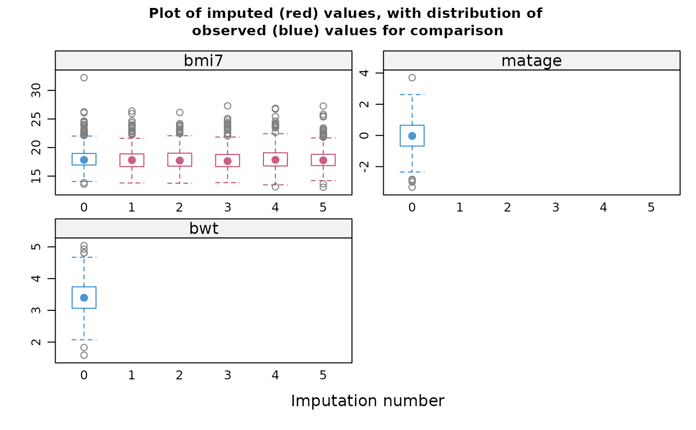
#> method = c( ‘norm’ ) # Specify a method for each incomplete variable.
#> If displayed, the box-and-whisker plots can be used to inform your
#> choice of method(s): for example, if the imputation model does not
#> predict extreme values appropriately, consider a different imputation
#> model/method e.g. PMM. Note the distribution of imputed and observed
#> values is displayed for numeric variables only. The distribution may
#> differ if data are missing at random or missing not at random. If you
#> suspect data are missing not at random, the plots can also inform your
#> choice of sensitivity parameter.
#>
#> formulas = formulas_list , # Note that you do not additionally need to
#> specify a 'predmatrix'
#>
#> # The formulas_list specifies the conditional imputation models, which
#> are as follows:
#>
#> ‘bmi7 ~ matage + I(matage^2) + mated + pregsize’
#>
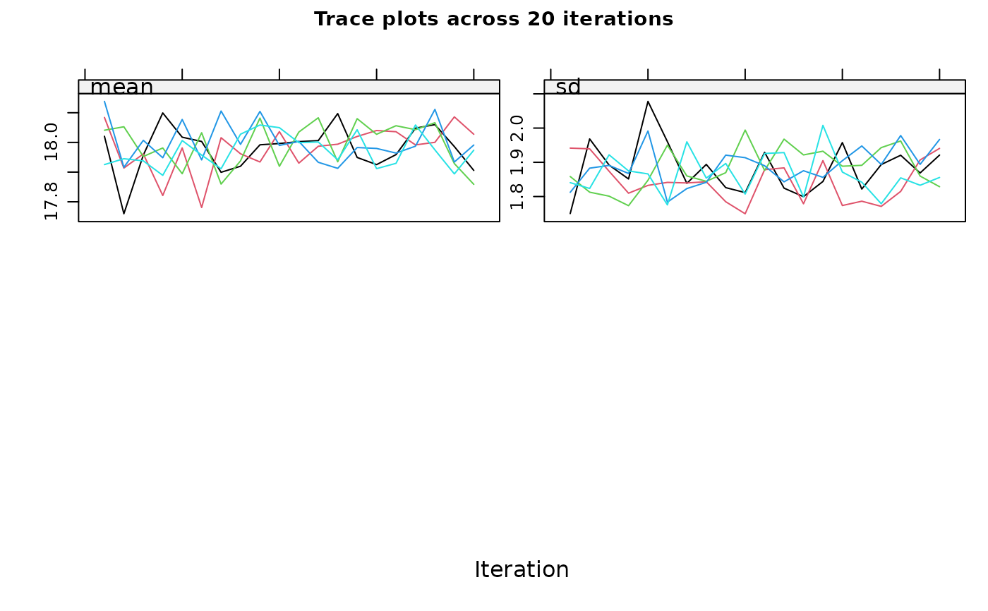
#> maxit = 10 , # If you have more than one incomplete variable, you
#> should check this number of iterations is sufficient by inspecting the
#> trace plots, if displayed. Consider increasing the number of iterations
#> if there is a trend that does not stabilise by the 10th iteration. Note
#> that iteration is not performed when only one variable is partially
#> observed.
#>
#> printFlag = FALSE , # Change to printFlag=TRUE to display the history
#> as imputation is performed
#>
#> seed = NA) # It is good practice to choose a seed so your results are
#> reproducible
# Display the proposed 'mice' options
## When specifying a single imputation model
proposeMI(mimodobj=mimod_bmi7,
data=bmi)
#> Based on your proposed imputation model and dataset, your mice() call
#> should be as follows:
#>
#> mice(data = bmi , # You may need to specify a subset of the columns in
#> your dataset; if you specified stratification variable(s) in your
#> proposed imputation model(s), these will be carried over to 'midoc'
#> functions 'doMImice' and 'doMNARmice' and multiple imputation will be
#> performed for each subset of the data determined by the values of the
#> stratification factor(s)
#>
#> m = 41 , # You should use at least this number of imputations based on
#> the proportion of complete records in your dataset
#>
#> method = c( ‘norm’ ) # Specify a method for each incomplete variable.
#> If displayed, the box-and-whisker plots can be used to inform your
#> choice of method(s): for example, if the imputation model does not
#> predict extreme values appropriately, consider a different imputation
#> model/method e.g. PMM. Note the distribution of imputed and observed
#> values is displayed for numeric variables only. The distribution may
#> differ if data are missing at random or missing not at random. If you
#> suspect data are missing not at random, the plots can also inform your
#> choice of sensitivity parameter.
#>
#> formulas = formulas_list , # Note that you do not additionally need to
#> specify a 'predmatrix'
#>
#> # The formulas_list specifies the conditional imputation models, which
#> are as follows:
#>
#> ‘bmi7 ~ matage + I(matage^2) + mated + pregsize’
#>
#> maxit = 10 , # If you have more than one incomplete variable, you
#> should check this number of iterations is sufficient by inspecting the
#> trace plots, if displayed. Consider increasing the number of iterations
#> if there is a trend that does not stabilise by the 10th iteration. Note
#> that iteration is not performed when only one variable is partially
#> observed.
#>
#> printFlag = FALSE , # Change to printFlag=TRUE to display the history
#> as imputation is performed
#>
#> seed = NA) # It is good practice to choose a seed so your results are
#> reproducible
 ## When specifying more than one imputation model (suppressing the plots)
proposeMI(mimodobj=list(mimod_bmi7,mimod_pregsize),
data=bmi,
plot=FALSE)
#> Based on your proposed imputation model and dataset, your mice() call
#> should be as follows:
#>
#> mice(data = bmi , # You may need to specify a subset of the columns in
#> your dataset; if you specified stratification variable(s) in your
#> proposed imputation model(s), these will be carried over to 'midoc'
#> functions 'doMImice' and 'doMNARmice' and multiple imputation will be
#> performed for each subset of the data determined by the values of the
#> stratification factor(s)
#>
#> m = 41 , # You should use at least this number of imputations based on
#> the proportion of complete records in your dataset
#>
#> method = c( ‘norm’, ‘logreg’ ) # Specify a method for each incomplete
#> variable. If displayed, the box-and-whisker plots can be used to
#> inform your choice of method(s): for example, if the imputation model
#> does not predict extreme values appropriately, consider a different
#> imputation model/method e.g. PMM. Note the distribution of imputed and
#> observed values is displayed for numeric variables only. The
#> distribution may differ if data are missing at random or missing not at
#> random. If you suspect data are missing not at random, the plots can
#> also inform your choice of sensitivity parameter.
#>
#> formulas = formulas_list , # Note that you do not additionally need to
#> specify a 'predmatrix'
#>
#> # The formulas_list specifies the conditional imputation models, which
#> are as follows:
#>
#> ‘bmi7 ~ matage + I(matage^2) + mated + pregsize’
#>
#> ‘pregsize ~ bmi7 + matage + I(matage^2) + mated’
#>
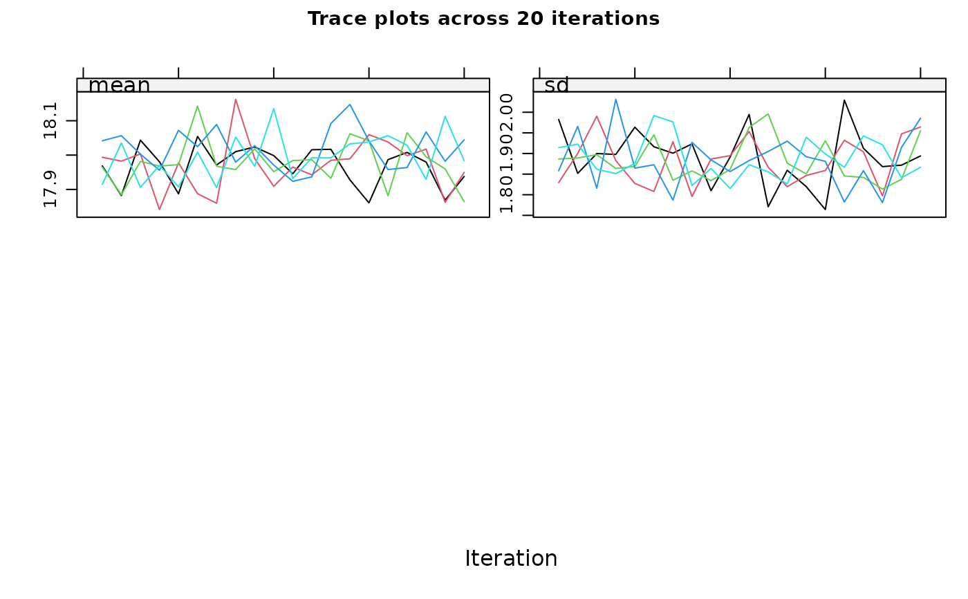
#> maxit = 10 , # If you have more than one incomplete variable, you
#> should check this number of iterations is sufficient by inspecting the
#> trace plots, if displayed. Consider increasing the number of iterations
#> if there is a trend that does not stabilise by the 10th iteration. Note
#> that iteration is not performed when only one variable is partially
#> observed.
#>
#> printFlag = FALSE , # Change to printFlag=TRUE to display the history
#> as imputation is performed
#>
#> seed = NA) # It is good practice to choose a seed so your results are
#> reproducible
## When specifying more than one imputation model (suppressing the plots)
proposeMI(mimodobj=list(mimod_bmi7,mimod_pregsize),
data=bmi,
plot=FALSE)
#> Based on your proposed imputation model and dataset, your mice() call
#> should be as follows:
#>
#> mice(data = bmi , # You may need to specify a subset of the columns in
#> your dataset; if you specified stratification variable(s) in your
#> proposed imputation model(s), these will be carried over to 'midoc'
#> functions 'doMImice' and 'doMNARmice' and multiple imputation will be
#> performed for each subset of the data determined by the values of the
#> stratification factor(s)
#>
#> m = 41 , # You should use at least this number of imputations based on
#> the proportion of complete records in your dataset
#>
#> method = c( ‘norm’, ‘logreg’ ) # Specify a method for each incomplete
#> variable. If displayed, the box-and-whisker plots can be used to
#> inform your choice of method(s): for example, if the imputation model
#> does not predict extreme values appropriately, consider a different
#> imputation model/method e.g. PMM. Note the distribution of imputed and
#> observed values is displayed for numeric variables only. The
#> distribution may differ if data are missing at random or missing not at
#> random. If you suspect data are missing not at random, the plots can
#> also inform your choice of sensitivity parameter.
#>
#> formulas = formulas_list , # Note that you do not additionally need to
#> specify a 'predmatrix'
#>
#> # The formulas_list specifies the conditional imputation models, which
#> are as follows:
#>
#> ‘bmi7 ~ matage + I(matage^2) + mated + pregsize’
#>
#> ‘pregsize ~ bmi7 + matage + I(matage^2) + mated’
#>
#> maxit = 10 , # If you have more than one incomplete variable, you
#> should check this number of iterations is sufficient by inspecting the
#> trace plots, if displayed. Consider increasing the number of iterations
#> if there is a trend that does not stabilise by the 10th iteration. Note
#> that iteration is not performed when only one variable is partially
#> observed.
#>
#> printFlag = FALSE , # Change to printFlag=TRUE to display the history
#> as imputation is performed
#>
#> seed = NA) # It is good practice to choose a seed so your results are
#> reproducible